Survival Analysis 
A little bit about me 
- Data Analyst @ Autodesk
- You can find me at RaulingAverage.dev
- Enjoy Coffee, Learning, and Running..near the beach
Notes:
- This presentation does not reflect any workings or material from Autodesk
And I am not a core-contributor to the Lifelines project, but a user
I hope you and your families are well during these times! Moreover, please be safe as I encourage y’all to Social Distance, Wear Masks, Wash Hands, and of course be well. #Masks4All
What will we be talking about today? 
What is Survival Analysis? 
Survival Analysis is used to estimate the time of event of interest for some sample or population. In it’s origination through medical research, one would like to understand the time of death, as random variable time T goes on. Since it's origination, the analysis has been used in other applications like customer churn, error logging, or mechanical failure.
As a summary: “Survival analysis attempts to answer questions such as: what is the proportion of a population which will survive past a certain time? Of those that survive, at what rate will they die or fail?” - Source
Say we have database of Insta2U customers and their subscriptions,a fake a delivery service company for 2U albums. This database has start & ending of subscription dates, and the customer's associated features/signals.
churn_dataSample.head()
Because of the start and end date of these customer, we can observe these customer's life expectancies (or their churn) over time t, seen below:
Moreover, there are nice properties of this implementation we can utilize to ensure we have an accurate depiction of observing the event of interest, in our case churn, over time.
Look at Table 5. First it's amazing to see a paper w/ >1,100 vented #Covid19 pts. But of these 1151 vented pts, *at a median follow-up time of 4.5d* only 38 went home, 282 died, while 831 were still hospitalized. 282/(38+282) = 88% mortality. But thats *quite* misleading👇(4/x) pic.twitter.com/za3S6qEBFj
— John W Scott, MD MPH (@DrJohnScott) April 23, 2020
What are those special properties? 
Censoring 
If we look at the following image, we observe one case where people have not experiences some occurence, and continue to persist. If we take the mean of these data points, we are underestimate the average because those who continue to stay alive after time t, skew our average.
And if we only consider one segmentation of individuals, say those who had their event of occurence happen, we too still underestimate our average of the values.
So, it solves the problem of right-censoring, mentioned later. Even with no censoring, this analysis is still great for understanding time and events of interest.
from lifelines.plotting import plot_lifetimes

ax = plot_lifetimes(churn_dataSample['tenure'],event_observed = churn_dataSample['Churn - Yes'])
ax.vlines(50, 0, 50, linestyles='--')
ax.set_xlabel("time")
ax.set_title("Customer Tenure, at t=50")

Probabilities over Time 
Survival Function
The survival function $S(t)$ estimates the probability of surviving past some time $t$, for the observations going to $t \rightarrow \infty$.
As a definition:
For $T$ be a non-negative random lifetime taken from the population, the survival function $S(t)$ is defined as
$$S(t) = \text{Pr}(T>t) = 1-F(t)$$where $T$ is the response variable, where $T \geq 0$
Including it's properties
- As t ranges from $0$ to $\infty$, the survival function has the following properties;
- $S(t)$ is Non-increasing
- At t=0, S(t) = 1. In other words, the probability of surviving past time $t= 0$ is 1.
- Moreover, At t=$\infty$, $S(t) = S(\infty)=0$. As time goes to infinity, survival curve goes to 0.
- $0\leq S(t)\leq 1$
- $F_T(t) = 1 - S(t)$, where $F_T(t)$ is a "Cumaltive Density function"
Regression 
Survival regression allows us to regress other feature against another variable--this case durations. This regression is particularly different in that:
- It abides to characteristic of censoring, compared to traditional Linear Regression
- Though it can operate like traditional linear regression, itt is used to explore the relationship between the 'survival' of person and characteristics
- Predict the survivability through the model, as opposed to predicting estimations
- All models attempt to represent the hazard rate $h(t|x_i)$ for some $i=1....n$
- Cox’s proportional hazard model
- Aalen’s additive model
- Exponential
And more! 
Okay, I'm convinced. How can we implement this process? 


- Lifelines is a Python package for Survival Analysis created by Cam Davidson Pilon during his time as a Director of Decision Science at Shopify
from lifelines import KaplanMeierFitter
Benefits:
- SciKit-Learn friendly
- Built on top of Pandas
- Only focus is survival analysis
- Handles right, left and interval censored data
- Estimating Hazard Rates
- Defining personal Survival Models
- Compare two or more survival functions
lifelines.statistics.logrank_test()
- and more!
Kaplan-Meier Estimate & S(t)
How is the S(t) calculated? Kaplan-Meier Estimation
Kaplan-Meier Estimation allows us to create an algorithm to calculate $S(t)$.
We calculate the Survival Function through the following formula:
$\hat{S(t)} = \prod_{t_i < t} \tfrac{n_i-d_i}{n_i}$
where $d_i$ are the number of death events at time $t$ and $n_i$ is the number of subjects at risk of death just prior to time $t$.
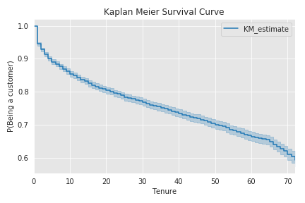
Let's look at our Customer Churn scenario, and apply it as an example using this Customer dataset from the Lifelines example workbooks.

from lifelines import KaplanMeierFitter
kmf = KaplanMeierFitter()

kmf.fit(durations = churn_data['tenure'], event_observed = churn_data['Churn - Yes'])
kmf.plot(ci_show=True)
plt.title('Kaplan Meier Survival Curve')
plt.ylabel('P(Being a customer)')
plt.xlabel('Tenure')
plt.tight_layout()
plt.savefig(firstDemoImage)
plt.show()

print("We output the Event occurence table over time 'event_at'")

kmf.event_table.head()
print("As another part of the functionality with Lifelines are" +
      "conveniently printing out statistical information as Dataframes")
kmf.confidence_interval_.head()
What about Regression?
An example of this implementation will be covered in a future talk.
However, there are example of implementing Survival Regression in the Lifelines documentation.
With that being said 

Resources
There is an R implementation called Survival
- There is a Sci-kit Learn equivalent called Scikit-Survival