Survival Analysis 
A little bit about me 
- Data Analyst @ Autodesk & Teaching Fellow @ Delta Analytics
- You can find me at RaulingAverage.dev
- Enjoy Coffee, Learning, and Running..near the beach
Notes:
- This presentation does not reflect any workings or material from Autodesk
And I am not a core-contributor to the Lifelines project, but a user
I hope you and your families are well during these times! Moreover, please be safe as I encourage y’all to Social Distance, Wear Masks, and contribute to social movements during these next critical months.
What will we be talking about today? 
What is Survival Analysis? 
Survival Analysis is an analytics process to estimate the time of event of interest for some group, sample, or population.

In it’s origination through medical research, one would like to understand the time of an "event of interest" will occur, in consideration of time t. Since it's origination, the analysis has been used in other applications like customer churn, error logging, or mechanical failure.
As a summary, “Survival analysis attempts to answer questions such as:
What is the proportion of a population which will survive past a certain time? Of those that survive, at what rate will they die or fail?” - Source
churn_dataSample.head(3)
- If we take the mean $\bar{x}$, all data points considered, we underestimate the true average because of those who continue to stay alive after time t, they skew our average customer lifespan.
print(f"Average Tenure for customers, all data points considered: {churn_dataSample['tenure'].mean()}")
However, what about cases where individuals may:
- Come in later into the study than other participants?
- Drop off earlier from other participants?
- Continue to be present after the study is conducted?
- Take time in showing results, considering a deadline?
Wouldn't this improperly represent our estimated customer lifespans?
In the coding section later on, we will see that we can visualize an accurate depication of these customer's life expectancies (or churn) over time t, seen below:
Look at Table 5. First it's amazing to see a paper w/ >1,100 vented #Covid19 pts. But of these 1151 vented pts, *at a median follow-up time of 4.5d* only 38 went home, 282 died, while 831 were still hospitalized. 282/(38+282) = 88% mortality. But thats *quite* misleading👇(4/x) pic.twitter.com/za3S6qEBFj
— John W Scott, MD MPH (@DrJohnScott) April 23, 2020
Side note: If you want to follow some reliable epidemiologists I recommend the following Twitter handles:
@DrTomFrieden @EpiEllie @DrEricDing @DWUhlfelderLaw @ASlavitt @CT_Bergstrom
This case of misinterpreting #COVID19 values without the consideration of time or condition can miscontrue our results.
Hence why this talk isn't more focused on using healthcare or epidemiology data
Now, we briefly go over some interesting properties of this implementation 
Censoring 
A form of missing data problem in which time to event is not observed for reasons:
- Early termination in study
- Subject has left the study prior to experiencing an event
- Subject continues to not experience event of interest, after study ends
Censoring allows for considering time-based data problems with inclusion of event of interests, and moreover other factors.
The following is a visualization and expansion of what types of Censoring exist:
from lifelines.plotting import plot_lifetimes

ax = plot_lifetimes(churn_dataSample['tenure'],
                    event_observed = churn_dataSample['Churn - Yes']
                   )
ax.vlines(50, 0, 50, linestyles='--')
ax.set_xlabel("Time")
ax.set_ylabel("Person")
ax.set_title("Customer Tenure, at t=50")

There are two types of censoring.
Right Censoring:
- Setting the max lifespan value at time t for data points that would go beyond time *t
Se the first top 5 lines for those data points who do go beyond some times t, but are right censored in the calculations
Left Censoring:
- Consideration of data points with no start time, in cases where no "start" timeframe was originally found.
Note: Useful in cumulative density calculations.
If we calculate a statistic, like average, for either:
- groups with no occurence of event of interest, after the study
- groups that quite experience an event of interest before the study ends
- or when a person comes later into the sample group timeframe
Then we would tend to underestimate our results.
So, the consideration of censoring both an effective and crucial part of Survival Analysis
Probabilities over Time 
Survival Function
The survival function $S(t)$ estimates the probability of surviving past some time $t$, for the observations going to $t \rightarrow \infty$.
As a definition:
For $T$ be a non-negative random lifetime taken from the population, the survival function $S(t)$ is defined as
$$S(t) = \text{Pr}(T>t) = 1-F(t)$$where $T$ is the response variable, where $T \geq 0$

Regression 
Survival regression allows us to regress other feature against another variable--this case durations. This type of regression is different from other common regressions in that:
- It abides to characteristic of Censoring
- Though it can operate like traditional linear regression, itt is used to explore the relationship between the 'survival' of person and characteristics
- All models attempt to represent the hazard rate $h(t|x_i)$ for some $i=1....n$
- Cox’s proportional hazard model
- Aalen’s additive model
- ...
And more! 
Okay, I'm convinced. How can we implement this process? 


- Lifelines is a Python package for Survival Analysis created by Cam Davidson Pilon during his time as a Director of Decision Science at Shopify
Benefits:
- SciKit-Learn friendly
- Pandas Experience
from lifelines import KaplanMeierFitter

## With some neat API usage...coming up
- Abstract away coding to focus on subject matter
- Handles different types of Interval Censored data
- Customization for analyses that either do not meet or are outside assumptions
- Compare two or more survival curves
lifelines.statistics.logrank_test()
- And more!
Kaplan-Meier Estimate & S(t)
Kaplan-Meier Estimation allows us to analyze data with event of interest for some time t.
We calculate the Survival Function $S(t)$ by the following formula:
$\hat{S(t)} = \prod_{t_i < t} \tfrac{n_i-d_i}{n_i}$
where $d_i$ are the number of death events at time $t$ and $n_i$ is the number of subjects at risk of death just prior to time $t$.
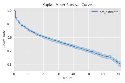
Let's look at our Customer Churn data, from the Lifelines example library, with the Kaplan-Meier implementation to estimate Survival Curve

from lifelines import KaplanMeierFitter
kmf = KaplanMeierFitter()
kmf.fit(durations = churn_data['tenure'], event_observed = churn_data['Churn - Yes'])
kmf.plot(ci_show=True)
# kmf.plot(ci_show=True, at_risk_counts=True)

plt.title('Kaplan Meier Survival Curve')
plt.ylabel('Survival Rate')
plt.xlabel('Tenure')
plt.tight_layout()
plt.savefig(firstDemoImage)
plt.show()

print("We output the Event occurence table over time 'event_at'")
kmf.event_table.head()
Remember that perceivably convoluted Kaplan Mier equation?
$\hat{S(t)} = \prod_{t_i < t} \tfrac{n_i-d_i}{n_i}$
Let's take a small sample of the first 3 rows to see how (readably) calculated:
event_atZero = (7043 - 0) / 7043
event_atOne = event_atZero * ((7032 - 380)/ 7032)
event_atTwo = event_atOne * ((6419 - 123)/ 6419)
demoEventsSurvival = [event_atZero, event_atOne, event_atTwo]
totalExamples = len(demoEventsSurvival)
for i in range(totalExamples):
    survivalRate_rounded = round(demoEventsSurvival[i], 5)
    print(f"Calculated S(t) = {survivalRate_rounded}, at timeline event_at = {i}")
Just to confirm our calculations...
print('The following are our S(t) estimation calculations from our Kaplan Meir object:\n')
kmf.survival_function_.head()
print("As another part of the functionality with Lifelines are" +
      "conveniently printing out statistical information as Dataframes\n")
kmf.confidence_interval_.head()

We notice that the Kaplan-Meir implementation focuses on categorical factors to produce the resulting Survival Rate Curve over time. Moreover, we were not able to do the following:
- include other variables within said calculation.
- associate some x to y result.
- control other confounding factors for measure impact on a feature
Cox Proportional Hazard Model
$$h(t|x) = b_o(t) \exp(\sum_{i=1}^n b_i (x_i - \bar{x_i}))$$- It is semi-parametric
- Can include other categorical/non-categorical factors
- Estimate hazard ratios from coefficients to gauge hazards $h(*)$ between groups
- Assumptions:
- Censoring is non-informative in calculations
- Individuals and events are independent
- X values do not change over time
- Proportional hazards are constant over time
from lifelines import CoxPHFitter

cox_saRegression = CoxPHFitter()
selectedFeatures = ['tenure','SeniorCitizen', 'MonthlyCharges', 'Churn - Yes']
cox_saRegression.fit(churn_data[selectedFeatures],
                     duration_col='tenure', event_col='Churn - Yes')

cox_saRegression.print_summary()
Note: If the Hazard Ratio is <1, then there is a lower hazard rate between some two groups. Else, it's higher.
cox_saRegression.plot()
plt.title('Confidence Interval for Cox Model')
plt.ylabel('Factors/Covariates')
plt.show()
cox_saRegression.summary

Plotting the effect of varying a covariate (factor)
To visbally understand the impact of a factor, we plot survival curves for varying covariate values, while holding everything else equal. This is useful to understand the impact of a factor, given the model.
covariateElement = 'SeniorCitizen'
cox_saRegression.plot_covariate_groups(covariates='SeniorCitizen', values=[0, 1], cmap='coolwarm')
plt.title(f'Covariate Example: Cox Model by Covariate {covariateElement}')
plt.xlabel('Time')
plt.ylabel('Survival Rate')
plt.show()

This is an introduction to Survival Regression, but what about cases when:
- Hazard Rate is not constant over time?
- Consider penalization of particular datasets influencing our data?
- And other considerable further conditions that may violate our Cox model's assumptions?
In that case, instead of using the Cox Proportion Model, we could use the Aaelen's model or other parametric or customized models from Lifelines!
You can more about this in the Lifelines documentation.
I would continue on, but I want us to get through and survive this talk. 

With that being said 
Thank you.... 

Resources
Survival Analysis
- Lifelines package by Cameron Davidson-Pilon
- Survival Analysis Overview via NCBI
- There is an R implementation called Survival
- There is a Sci-kit Learn equivalent called Scikit-Survival