All topics / SQL

SQL

Query writing, window functions, joins, and performance scenarios.

Filter by difficulty
Card 1 of 15 0 known
beginner

A data quality alert fires saying your trips table has more rows than unique trip_id values — commuters have reported the app double-logging trips whenever a spotty GPS signal triggers a sync retry. How do you quickly find which trip_ids are duplicated and how many times each appears?

  • #duplicates
  • #group-by
  • #data-quality
Click or press Enter to reveal the answer
Answer

Group by trip_id, count the rows in each group, and filter with HAVING count(*) > 1 — GROUP BY collapses rows into one per trip_id, and HAVING filters on that aggregated count, which a WHERE clause can't do since WHERE runs before aggregation happens.

The query

select
    trip_id,
    count(*) as row_count
from trips
group by trip_id
having count(*) > 1
order by row_count desc

Why HAVING and not WHERE

SQL evaluates clauses roughly in this order: FROMWHEREGROUP BYHAVINGSELECTORDER BY. WHERE filters individual rows before grouping happens, so at that point count(*) doesn’t exist yet — there’s nothing to filter on. HAVING filters after aggregation, once count(*) per group is known, which is exactly what you need to say “keep only the groups with more than one row.”

-- This does NOT work: count(*) isn't available at the WHERE stage
select trip_id
from trips
where count(*) > 1  -- error
group by trip_id

A quick sanity check without the full breakdown

If you just want a yes/no answer to “are there any duplicates at all” before digging into which ones:

select count(*) as total_rows, count(distinct trip_id) as unique_ids
from trips

If total_rows doesn’t equal unique_ids, duplicates exist — then run the GROUP BY ... HAVING query above to identify exactly which trip_ids are affected and by how much, which is the first step toward root-causing the upstream issue (in this case, the mobile app resending a trip after a failed GPS sync instead of recognizing it had already uploaded).

Click to flip back
beginner

A stakeholder wants a chart of weekly active bike commuters, but your trips table has a trip_date column logged at all different times of day across the week. How do you bucket that into weeks?

  • #date-functions
  • #time-series
Click or press Enter to reveal the answer
Answer

Truncate the trip date down to the week grain with DATE_TRUNC('week', trip_date), then GROUP BY the truncated value to count distinct commuters per week who logged a bike trip.

The query

select
    date_trunc('week', trip_date) as week_start,
    count(distinct commuter_id) as weekly_active_bike_commuters
from trips
where mode = 'bike'
group by date_trunc('week', trip_date)
order by week_start

DATE_TRUNC('week', ...) rounds every trip date down to the start of the week it falls in (e.g., every trip between Monday and Sunday collapses to the same Monday date), so grouping by the truncated value aggregates all bike trips within that week together.

Things to watch out for

  • Week start day varies by engine/locale. Postgres and Snowflake’s DATE_TRUNC('week', ...) default to Monday as the start of the week; some configurations or other functions default to Sunday. If a city partner’s reporting calendar uses a different week start, you may need DATE_TRUNC with an explicit anchor, or a manual bucketing expression, to match their expectations.
  • COUNT(DISTINCT commuter_id) is not additive across weeks. A commuter who bikes in both week 1 and week 2 gets counted once in each week individually, which is correct for weekly totals, but you cannot sum weekly numbers to get a monthly total — that requires a separate COUNT(DISTINCT commuter_id) grouped at the month grain.
  • Other common granularities follow the same pattern: date_trunc('day', ...), date_trunc('month', ...), date_trunc('quarter', ...). BigQuery uses the same DATE_TRUNC function name but with a slightly different argument order (DATE_TRUNC(trip_date, WEEK)), so double-check syntax per warehouse.

This pattern — truncate, then group by the truncated value — is the standard way to build any time-series aggregation for GreenMile’s dashboards, whether it’s daily signups, weekly active bike commuters, or monthly subsidy enrollments.

Click to flip back
beginner

GreenMile Mobility wants a list of commuters who created an account in the app but have never logged a single trip, pulling from a commuters table and a trips table. Walk me through how you'd write that query.

  • #anti-join
  • #not-exists
  • #joins
Click or press Enter to reveal the answer
Answer

Use an anti-join: either a LEFT JOIN from commuters to trips filtered on trips.commuter_id IS NULL, or a NOT EXISTS correlated subquery — both return commuters with no matching trip row. NOT EXISTS is often preferred because it short-circuits per row and avoids the classic NULL pitfall that NOT IN has.

Option 1: LEFT JOIN … IS NULL

select c.commuter_id, c.home_city
from commuters c
left join trips t on c.commuter_id = t.commuter_id
where t.commuter_id is null

The LEFT JOIN keeps every commuter row regardless of a match; for commuters with no logged trips, all columns from trips come back NULL. Filtering on t.commuter_id is null isolates exactly those non-matches.

Option 2: NOT EXISTS

select c.commuter_id, c.home_city
from commuters c
where not exists (
    select 1
    from trips t
    where t.commuter_id = c.commuter_id
)

NOT EXISTS is a correlated subquery — for each commuter row, it checks whether any trip row matches, and keeps the commuter only if none do. Most query optimizers turn this into essentially the same anti-join plan as the LEFT JOIN version, so performance is usually comparable on modern engines.

Why NOT EXISTS is often the safer default

The one to actively avoid is NOT IN with a subquery that could return NULLs:

-- DANGEROUS if trips.commuter_id can ever be NULL
select commuter_id from commuters
where commuter_id not in (select commuter_id from trips)

If even one row in the subquery returns a NULL commuter_id — say, a bike-share trip logged anonymously through a kiosk with no linked account — the entire NOT IN comparison becomes indeterminate for every row, and the query can silently return zero rows instead of the expected list. NOT EXISTS and LEFT JOIN ... IS NULL don’t have this problem, which is why they’re generally the safer, more predictable choice for anti-joins.

Click to flip back
beginner

Leadership wants "the top 3 commuters by total km biked this month" per city, but two commuters in the Austin program are tied for third place, and leadership wants both included. Which ranking window function do you reach for, and why?

  • #window-functions
  • #ranking
Click or press Enter to reveal the answer
Answer

Use RANK() instead of ROW_NUMBER(), since RANK() assigns the same rank to tied rows and then skips the next rank, so both tied commuters get rank 3 and are included when you filter for rank <= 3. ROW_NUMBER() would arbitrarily break the tie and only keep one of them.

The three ranking functions

  • ROW_NUMBER() — assigns a strictly increasing, unique integer to every row in a partition, even if values are tied. Ties are broken arbitrarily (or by whatever secondary order you specify).
  • RANK() — ties get the same rank, and the next rank skips ahead by the number of tied rows (1, 2, 2, 4).
  • DENSE_RANK() — ties get the same rank, but the next rank does not skip (1, 2, 2, 3).

Applied to the question

with commuter_km as (
    select commuter_id, city, sum(distance_km) as total_km_biked
    from trips
    where mode = 'bike'
    group by commuter_id, city
)

select
    city,
    commuter_id,
    total_km_biked,
    rank() over (partition by city order by total_km_biked desc) as km_rank
from commuter_km
qualify km_rank <= 3

If two Austin commuters are tied at 42 km for third place, RANK() gives them both rank 3, and both pass the <= 3 filter — exactly the “include both ties” behavior leadership asked for. ROW_NUMBER() would assign one of them rank 3 and the other rank 4, silently dropping one from the leaderboard.

When to use each

  • Use ROW_NUMBER() when you specifically want exactly N rows per group regardless of ties (e.g., “give me exactly one row per commuter” for deduplication).
  • Use RANK() when ties should be reported as tied, and it’s acceptable that the count returned might exceed N.
  • Use DENSE_RANK() when you want tied values to share a rank but don’t want gaps in the ranking sequence — useful for things like “top 3 distinct km-biked tiers” for a rewards program.

Note: QUALIFY (available in Snowflake and BigQuery) lets you filter on a window function result directly; in engines without it (e.g., Postgres), wrap the window function in a CTE and filter in an outer WHERE.

Click to flip back
beginner

You calculate AVG(cost_usd) across all trips to report the average cost of a GreenMile commute, and the number seems too high — then you realize walking trips have a NULL cost_usd because the app's cost calculator simply never runs for the "walk" mode, not because billing data is missing. What's happening, and how do you fix it?

  • #nulls
  • #aggregates
  • #joins
Click or press Enter to reveal the answer
Answer

AVG(), like all standard aggregate functions except COUNT(*), silently ignores NULL values rather than treating them as zero, so the average is really only being computed over car and bus trips, inflating the result. Fix it by explicitly coalescing NULLs to zero with COALESCE(cost_usd, 0) before averaging, since a walking trip genuinely costs nothing.

Why the average looked inflated

select avg(cost_usd) from trips

If 10,000 trips exist but 2,000 of them are walking trips with a NULL cost_usd, AVG() divides the sum by 8,000, not 10,000 — the 2,000 free walking trips are simply excluded from the calculation entirely, as if they didn’t exist. That’s correct behavior for “average cost among car and bus trips,” but not what leadership meant by “average cost across all commute trips.”

The fix

select avg(coalesce(cost_usd, 0)) as avg_trip_cost_all_modes
from trips

COALESCE(cost_usd, 0) replaces NULL with 0 before the average is computed, so now the denominator correctly reflects all 10,000 trips. This is the right fix specifically because a walking trip’s true cost is $0 — if the NULL instead meant “unknown, receipt not uploaded” (as it does for some car trips), coalescing to zero would understate the average instead of correcting it, so it’s worth confirming what a NULL actually represents for each mode before applying this pattern.

The same trap shows up in joins

NULLs also cause silent row loss in joins, because NULL = NULL never evaluates to true in standard SQL:

select t.trip_id, c.home_city
from trips t
join commuters c on t.commuter_id = c.commuter_id

If t.commuter_id is NULL for some anonymous bike-share trips logged through a public kiosk, those rows simply vanish from an inner join result — not because of an error, but because NULL never matches anything, including another NULL. If you need to keep those rows, a LEFT JOIN (and possibly a COALESCE or explicit “unlinked trip” placeholder) is required.

The general lesson

Before trusting any aggregate or join result, ask: “does this column ever contain NULL, and if so, does the default SQL behavior (ignore in aggregates, never match in joins) match what the business question actually means?” It’s a very common source of quietly wrong numbers that pass code review because the query runs without error.

Click to flip back
intermediate

HR at GreenMile Mobility wants a report listing every employee alongside their manager's name, from a single employees table that has an employee_id column and a manager_id column pointing back to another employee_id. How do you produce that?

  • #self-join
  • #hierarchy
Click or press Enter to reveal the answer
Answer

Self-join the employees table to itself, joining employee.manager_id to manager.employee_id, aliasing the two instances so you can select the employee's name from one side and the manager's name from the other.

The query

select
    e.employee_id,
    e.employee_name,
    m.employee_name as manager_name
from employees e
left join employees m
    on e.manager_id = m.employee_id

Both e and m refer to the exact same table, but the aliases let SQL treat them as two logically separate “roles” in the join: e represents “the employee,” m represents “that employee’s manager.” The join condition e.manager_id = m.employee_id finds the row in the manager role whose employee_id matches the employee’s manager_id.

Why LEFT JOIN, not INNER JOIN

Using LEFT JOIN instead of INNER JOIN ensures employees with no manager (at GreenMile, that’s the CEO or another top-level exec, whose manager_id is NULL) still appear in the results, just with manager_name as NULL, rather than being silently dropped from the report.

Extending to multi-level hierarchies

A single self-join only gets you one level up (employee → direct manager). If HR later asks for the full chain up to the CEO (employee → manager → manager’s manager → …), a single join won’t scale to arbitrary depth — that calls for a recursive CTE:

with recursive org_chart as (
    select employee_id, employee_name, manager_id, 1 as level
    from employees
    where manager_id is null

    union all

    select e.employee_id, e.employee_name, e.manager_id, oc.level + 1
    from employees e
    join org_chart oc on e.manager_id = oc.employee_id
)
select * from org_chart order by level, employee_id

The self-join pattern is the right tool for “one level of relationship within the same table”; recursive CTEs are the right tool once GreenMile needs to traverse an arbitrary number of levels, e.g. for a company-wide org chart as the team scales past a single layer of management.

Click to flip back
intermediate

Someone asks you to find the second-highest-cost trip per commuter, but warns you that some commuters have duplicate trip costs (e.g. the same parking fee logged twice). What approach avoids getting tripped up by ties or by misusing LIMIT/OFFSET?

  • #window-functions
  • #ranking
  • #edge-cases
Click or press Enter to reveal the answer
Answer

Use DENSE_RANK() partitioned by commuter and ordered by cost descending, then filter for rank = 2 — DENSE_RANK treats duplicate costs as sharing the same rank rather than skipping past the actual second-highest distinct value the way a naive LIMIT/OFFSET or ROW_NUMBER approach would.

The query

with ranked_trips as (
    select
        commuter_id,
        cost_usd,
        dense_rank() over (
            partition by commuter_id
            order by cost_usd desc
        ) as cost_rank
    from trips
)
select commuter_id, cost_usd
from ranked_trips
where cost_rank = 2

Why DENSE_RANK, specifically

Suppose a commuter has trip costs of [15, 15, 8, 3]. The intent of “second highest” is almost always “the second-highest distinct cost,” which is 8 here, not a second copy of 15.

  • ROW_NUMBER() would assign 1, 2, 3, 4 — row 2 would be the second $15 trip, incorrectly treated as “second highest,” even though it’s really tied for first.
  • RANK() would assign 1, 1, 3, 4 — there’s no rank 2 at all, so filtering for rank = 2 returns nothing.
  • DENSE_RANK() assigns 1, 1, 2, 3 — rank 2 correctly lands on 8, the actual second-highest distinct value.

Why not LIMIT/OFFSET per commuter

A naive approach like ORDER BY cost_usd DESC LIMIT 1 OFFSET 1 only works for a single commuter at a time — there’s no clean way to apply “skip 1, take 1” independently per commuter in one query without a window function or a correlated subquery/LATERAL join, both of which are more verbose and error-prone than the DENSE_RANK() CTE above. The window-function approach also naturally handles commuters with fewer than two distinct trip costs (they simply have no row where cost_rank = 2, rather than causing an error).

Click to flip back
intermediate

The daily-km-biked chart across the program is noisy day to day and leadership keeps asking about single-day blips that don't mean anything. How would you smooth it with a 7-day moving average in SQL?

  • #window-functions
  • #moving-average
Click or press Enter to reveal the answer
Answer

Use AVG(km_biked) OVER (ORDER BY trip_date ROWS BETWEEN 6 PRECEDING AND CURRENT ROW) to compute a trailing 7-day average for each row, which smooths out day-to-day noise while still reacting to real trend changes.

The query

with daily_km as (
    select
        trip_date,
        sum(distance_km) as km_biked
    from trips
    where mode = 'bike'
    group by trip_date
)

select
    trip_date,
    km_biked,
    avg(km_biked) over (
        order by trip_date
        rows between 6 preceding and current row
    ) as km_biked_7day_moving_avg
from daily_km
order by trip_date

ROWS BETWEEN 6 PRECEDING AND CURRENT ROW defines a window of exactly 7 rows: the current row plus the 6 rows before it. AVG() computed over that window at each row produces a trailing (not centered) 7-day moving average — the standard choice for operational dashboards since it only ever looks backward, never at “future” data relative to the row being computed.

Behavior at the start of the series

For the first six rows of the table, there aren’t 6 preceding rows available yet — the window simply shrinks to however many rows actually exist (row 1 averages just itself, row 2 averages rows 1-2, etc.), rather than erroring or returning NULL. This is standard, well-defined window function behavior, but it’s worth flagging to stakeholders that the moving average for the very start of the program’s history is based on fewer than 7 days and will look artificially close to the raw daily value.

ROWS vs. RANGE

ROWS counts a fixed number of physical rows, which is what you want for “the last 7 calendar days” as long as there’s exactly one row per day with no gaps. If some days are missing from daily_km entirely (e.g., no bike trips logged anywhere on a holiday), ROWS BETWEEN 6 PRECEDING would actually span more than 7 calendar days to find 7 rows. RANGE BETWEEN INTERVAL '6 days' PRECEDING AND CURRENT ROW (supported in some engines like Postgres) instead defines the window in terms of actual date values, correctly spanning a true 7-calendar-day window regardless of gaps — worth reaching for if the data isn’t guaranteed to have one row per day.

Click to flip back
intermediate

The sustainability team wants a report showing, for each day, the cumulative CO2 saved (versus a driving baseline) for the month to date for each commuter, alongside that day's individual CO2 saved. How would you write this?

  • #window-functions
  • #running-total
Click or press Enter to reveal the answer
Answer

Use a window function: SUM(co2_saved_kg) OVER (PARTITION BY commuter_id, month ORDER BY day_date ROWS BETWEEN UNBOUNDED PRECEDING AND CURRENT ROW) to get a running total per commuter that resets at the start of each month.

The query

select
    commuter_id,
    day_date,
    date_trunc('month', day_date) as month,
    co2_saved_kg,
    sum(co2_saved_kg) over (
        partition by commuter_id, date_trunc('month', day_date)
        order by day_date
        rows between unbounded preceding and current row
    ) as co2_saved_month_to_date
from daily_co2_savings
order by commuter_id, day_date

How the frame clause works

  • PARTITION BY commuter_id, date_trunc('month', day_date) resets the running total at the start of each new month for each commuter — without it, the sum would accumulate across every commuter and every month with no reset.
  • ORDER BY day_date defines the order rows accumulate in; the running total at any row is the sum of all rows from the start of the partition up through the current one.
  • ROWS BETWEEN UNBOUNDED PRECEDING AND CURRENT ROW explicitly defines the window frame: “every row from the first row of the partition through the current row.” This is actually the default frame when ORDER BY is present without an explicit frame clause in most engines, but writing it out explicitly makes the intent unambiguous and protects against engine-specific default differences.

A subtlety worth knowing

If you omit the frame clause entirely and just write ORDER BY day_date with no ROWS BETWEEN, most engines default to RANGE BETWEEN UNBOUNDED PRECEDING AND CURRENT ROW — which behaves the same as ROWS here unless there are duplicate values in the ORDER BY column, in which case RANGE includes all peer rows (rows with the same value) in a single frame, potentially double-counting or under-splitting CO2 savings on days that share the same day_date for a commuter. Being explicit with ROWS BETWEEN avoids that ambiguity, especially useful if daily_co2_savings isn’t guaranteed to have exactly one row per commuter per day.

Click to flip back
intermediate

You have a mode column on the trips table with values like "car," "bike," and "bus," and leadership wants one row per commuter per month with a separate column for the count of trips taken by each mode. How do you pivot this in standard SQL?

  • #pivot
  • #case-when
Click or press Enter to reveal the answer
Answer

Use conditional aggregation: GROUP BY commuter_id and month, and for each mode write a SUM(CASE WHEN mode = 'x' THEN 1 ELSE 0 END) column — this works in any SQL dialect without needing a database-specific PIVOT operator.

The query

select
    commuter_id,
    date_trunc('month', trip_date) as trip_month,
    sum(case when mode = 'car'  then 1 else 0 end) as car_trip_count,
    sum(case when mode = 'bike' then 1 else 0 end) as bike_trip_count,
    sum(case when mode = 'bus'  then 1 else 0 end) as bus_trip_count
from trips
group by commuter_id, date_trunc('month', trip_date)

Each CASE WHEN expression evaluates to 1 if the row matches that mode and 0 otherwise; SUM() across the group then effectively counts how many trips of each mode occurred for that commuter-month. This is often called “conditional aggregation” and is the most portable way to pivot rows into columns — it works identically in Postgres, Snowflake, BigQuery, Redshift, and MySQL.

Native PIVOT as an alternative

Some warehouses offer a dedicated PIVOT clause that can express the same thing more concisely:

-- Snowflake-style PIVOT
select *
from trips
pivot(count(mode) for mode in ('car', 'bike', 'bus'))

Native PIVOT syntax varies meaningfully between warehouses (Snowflake, BigQuery, and SQL Server all have different syntax, and Postgres has none built in), which makes it less portable across environments. The CASE WHEN + SUM()/COUNT() approach is usually the safer default for anything that might need to run on more than one engine, or for a dbt project where the model might get ported later.

A useful variant: COUNT instead of SUM

If you only care about presence/absence rather than a count of occurrences, COUNT(CASE WHEN mode = 'x' THEN 1 END) (letting the ELSE implicitly be NULL, which COUNT ignores) works just as well and reads slightly cleaner.

Click to flip back
intermediate

You inherit a 200-line query full of deeply nested subqueries that computes total driving cost per city and is nearly impossible to debug. How would you refactor it, and is there ever a real performance reason to prefer one approach over the other?

  • #ctes
  • #subqueries
  • #sql-style
Click or press Enter to reveal the answer
Answer

Refactor into CTEs (WITH clauses), breaking the logic into named, sequential steps that are far easier to read, test, and debug independently. Performance-wise, most modern warehouses optimize CTEs the same as subqueries, so the choice is mostly about readability rather than speed.

Before: nested subqueries

select city, total_driving_cost
from (
    select city, sum(cost_usd) as total_driving_cost
    from (
        select t.city, t.cost_usd
        from trips t
        where t.mode = 'car'
    ) car_trips
    group by city
) city_totals
where total_driving_cost > 5000

Reading this inside-out to understand the logic is genuinely difficult, and adding a debug SELECT * on any intermediate step requires copy-pasting the nested block out separately.

After: CTEs

with car_trips as (
    select city, cost_usd
    from trips
    where mode = 'car'
),

city_totals as (
    select city, sum(cost_usd) as total_driving_cost
    from car_trips
    group by city
)

select city, total_driving_cost
from city_totals
where total_driving_cost > 5000

Each step is named for what it represents, reads top-to-bottom in the order the logic actually flows, and can be debugged independently just by changing the final SELECT to point at an earlier CTE — useful when a city’s driving cost total looks wrong and you need to check whether car_trips itself is pulling the right rows before trusting the aggregation on top of it.

The performance question

On modern optimizers (Snowflake, BigQuery, Redshift, Postgres 12+), CTEs are typically inlined — the query planner treats them the same as an equivalent subquery and optimizes across the whole query, so there’s usually no performance penalty for using them.

The historical exception is Postgres before version 12, where CTEs were always materialized (computed once into a temporary result and never re-optimized against the rest of the query) — which could occasionally help performance (by avoiding recomputation) but could also hurt it (by preventing the optimizer from pushing filters into the CTE). If you’re on an older Postgres version, this is worth checking; on essentially every modern cloud warehouse, prefer CTEs for readability without worrying about a performance tradeoff.

Click to flip back
advanced

Product wants a month-1, month-2, month-3 retention curve for the bike-to-work subsidy program by signup cohort — what percentage of commuters who signed up in a given month were still logging bike trips N months later. How would you structure this query?

  • #cohort-analysis
  • #retention
Click or press Enter to reveal the answer
Answer

First build a cohort table mapping each commuter to their signup month, then join to trips filtered to bike-mode to compute the month offset between signup and each active month, and finally aggregate the count of distinct active commuters per (cohort_month, month_offset) divided by the cohort's total signups.

Step 1: define each commuter’s cohort

with cohorts as (
    select
        commuter_id,
        date_trunc('month', signup_date) as cohort_month
    from commuters
),

Step 2: get each commuter’s distinct active bike months

bike_activity as (
    select distinct
        commuter_id,
        date_trunc('month', trip_date) as active_month
    from trips
    where mode = 'bike'
),

Step 3: compute month offset and join

cohort_activity as (
    select
        c.cohort_month,
        c.commuter_id,
        datediff('month', c.cohort_month, a.active_month) as month_offset
    from cohorts c
    join bike_activity a on c.commuter_id = a.commuter_id
    where a.active_month >= c.cohort_month
),

cohort_sizes as (
    select cohort_month, count(distinct commuter_id) as cohort_size
    from cohorts
    group by cohort_month
)

Step 4: aggregate into the retention curve

select
    ca.cohort_month,
    ca.month_offset,
    count(distinct ca.commuter_id) as retained_commuters,
    cs.cohort_size,
    round(100.0 * count(distinct ca.commuter_id) / cs.cohort_size, 1) as retention_pct
from cohort_activity ca
join cohort_sizes cs on ca.cohort_month = cs.cohort_month
group by ca.cohort_month, ca.month_offset, cs.cohort_size
order by ca.cohort_month, ca.month_offset

Reading the result

Each row answers “of commuters who signed up in cohort_month, what fraction were still logging bike trips month_offset months later?” month_offset = 0 should always be 100% (everyone was active in their own signup month, by definition of having logged a bike trip then), and the percentage should generally decay as month_offset increases. Plotting retention_pct against month_offset with one line per cohort_month is the standard cohort retention curve visualization — it’s exactly how GreenMile tells whether a bike-to-work subsidy is producing lasting behavior change versus a short-lived bump that fades within a month or two.

Click to flip back
advanced

The growth team wants to know which marketing channel should get credit for each commuter who eventually enrolls in the bike subsidy program — first touch or last touch — and asks you to build both views from a raw touchpoints table. How do you write each?

  • #attribution
  • #marketing-analytics
Click or press Enter to reveal the answer
Answer

First-touch attribution takes the earliest touchpoint per enrolled commuter (ROW_NUMBER ordered by timestamp ascending, filtered to rn = 1), while last-touch takes the most recent touchpoint before enrollment (ordered descending, filtered to rn = 1) — the same pattern, just flipping the sort direction of the ranking window function.

First-touch attribution

with ranked_touches as (
    select
        t.commuter_id,
        t.channel,
        t.touch_timestamp,
        row_number() over (
            partition by t.commuter_id
            order by t.touch_timestamp asc
        ) as touch_rank
    from touchpoints t
    join subsidy_enrollments e
        on t.commuter_id = e.commuter_id
        and t.touch_timestamp <= e.enrollment_timestamp
)
select commuter_id, channel as first_touch_channel
from ranked_touches
where touch_rank = 1

Last-touch attribution

with ranked_touches as (
    select
        t.commuter_id,
        t.channel,
        t.touch_timestamp,
        row_number() over (
            partition by t.commuter_id
            order by t.touch_timestamp desc
        ) as touch_rank
    from touchpoints t
    join subsidy_enrollments e
        on t.commuter_id = e.commuter_id
        and t.touch_timestamp <= e.enrollment_timestamp
)
select commuter_id, channel as last_touch_channel
from ranked_touches
where touch_rank = 1

The only structural difference is ASC vs DESC in the ORDER BY inside the window function — first-touch wants the earliest qualifying touchpoint (say, a social_ad impression), last-touch wants the most recent one (say, an employer_email reminder right before enrollment), and both filter to touch_rank = 1 to pick exactly one winning touchpoint per enrolled commuter. The join condition t.touch_timestamp <= e.enrollment_timestamp is what ensures you only consider touchpoints that happened before (or at) enrollment, not touchpoints from after the commuter already enrolled.

Why this is a starting point, not the whole answer

Both models are single-touch: they give 100% of the credit to one touchpoint and ignore every other channel the commuter interacted with along the way — a city_partnership flyer, an employer_email, and a social_ad might all have played a role before someone enrolled. This is simple and easy to compute, but it systematically overstates whichever channel tends to appear first (e.g., a city partnership campaign, if that’s usually a commuter’s entry point) or last (e.g., the employer email nudge, which often precedes an immediate enrollment). A natural extension is multi-touch attribution — linear (split credit evenly across all touches), time-decay (weight recent touches more), or U-shaped (extra weight on first and last) — each computed with a similar windowing pattern but distributing a fractional credit value across all rows instead of picking a single winner.

Click to flip back
advanced

You have a daily summary table built from trips showing whether each commuter logged a bike trip on a given day, and you need to identify continuous streaks of consecutive biking days per commuter — grouping them into a single streak. How do you solve this classic "gaps and islands" problem in SQL?

  • #gaps-and-islands
  • #window-functions
Click or press Enter to reveal the answer
Answer

Use the difference-of-sequences trick: rank each commuter's biking days by date, subtract that rank from the actual day number, and rows within the same continuous streak will land on the same constant value, which you can then GROUP BY to collapse each island into one row with a start and end date.

The intuition

If a commuter bikes on consecutive calendar days, both the day number and the row’s rank (1, 2, 3, …) increase by exactly 1 each time. Subtracting rank from the date therefore produces the same constant value for every day within one continuous streak, and a different constant for the next streak after any gap. That constant becomes a natural grouping key for each “island.”

The query

with bike_days as (
    select
        commuter_id,
        activity_date,
        row_number() over (
            partition by commuter_id
            order by activity_date
        ) as rn
    from commuter_daily_mode
    where logged_bike_trip = true
),

islands as (
    select
        commuter_id,
        activity_date,
        dateadd(day, -rn, activity_date) as island_key
    from bike_days
)

select
    commuter_id,
    min(activity_date) as streak_start,
    max(activity_date) as streak_end,
    count(*) as streak_length_days
from islands
group by commuter_id, island_key
order by commuter_id, streak_start

Walking through why it works

For a commuter biking Mon-Wed, skipping Thu, then biking again Sat-Sun:

activity_daternisland_key (date - rn days)
Mon1Sun (constant A)
Tue2Sun (constant A)
Wed3Sun (constant A)
Sat4Tue (constant B)
Sun5Tue (constant B)

Mon-Wed all subtract down to the same island_key, and Sat-Sun subtract down to a different one — so grouping by (commuter_id, island_key) correctly produces two separate streaks: Mon-Wed and Sat-Sun, with the Thursday gap correctly splitting them.

This same pattern generalizes to any “find continuous runs” problem — consecutive biking-streak achievements for a gamified subsidy program, uninterrupted days of subsidy eligibility, or continuous months of employer enrollment — by swapping the date arithmetic for whatever sequential unit defines the streak.

Click to flip back
advanced

You need to measure conversion through GreenMile's commute-program funnel — app signup, logging a first trip, enrolling in the employer bike subsidy, becoming a repeat bike commuter — per commuter, and the steps must happen in order. How do you compute step-by-step conversion rates?

  • #funnel-analysis
  • #conversion
Click or press Enter to reveal the answer
Answer

For each commuter, find the earliest timestamp of each funnel step using conditional MIN(), then require each step's timestamp to be after the previous step's to enforce ordering, and finally count how many commuters reached each step to compute conversion rates between steps.

Step 1: pivot each commuter’s step timestamps

with commuter_steps as (
    select
        commuter_id,
        min(case when event_name = 'signed_up'            then event_timestamp end) as signed_up_ts,
        min(case when event_name = 'first_trip_logged'     then event_timestamp end) as first_trip_ts,
        min(case when event_name = 'subsidy_enrolled'      then event_timestamp end) as subsidy_enrolled_ts,
        min(case when event_name = 'repeat_bike_commuter'  then event_timestamp end) as repeat_commuter_ts
    from commuter_events
    group by commuter_id
),

Using MIN() per step captures the first time each event happened for the commuter, which matters if, say, subsidy_enrolled fires more than once due to a re-enrollment.

Step 2: enforce ordering

ordered_funnel as (
    select
        commuter_id,
        signed_up_ts,
        case
            when first_trip_ts > signed_up_ts then first_trip_ts
        end as valid_first_trip_ts,
        case
            when subsidy_enrolled_ts > first_trip_ts
             and first_trip_ts > signed_up_ts
            then subsidy_enrolled_ts
        end as valid_subsidy_enrolled_ts,
        case
            when repeat_commuter_ts > subsidy_enrolled_ts
             and subsidy_enrolled_ts > first_trip_ts
             and first_trip_ts > signed_up_ts
            then repeat_commuter_ts
        end as valid_repeat_commuter_ts
    from commuter_steps
    where signed_up_ts is not null
)

This step matters because without it, a commuter who became a “repeat bike commuter” under an old program and only signed up for the current app much later (out of order, or across unrelated flows) would be incorrectly counted as a full funnel completion.

Step 3: compute step-by-step conversion

select
    count(signed_up_ts) as step1_signed_up,
    count(valid_first_trip_ts) as step2_first_trip_logged,
    count(valid_subsidy_enrolled_ts) as step3_subsidy_enrolled,
    count(valid_repeat_commuter_ts) as step4_repeat_bike_commuter,
    round(100.0 * count(valid_first_trip_ts) / count(signed_up_ts), 1) as pct_step1_to_step2,
    round(100.0 * count(valid_subsidy_enrolled_ts) / nullif(count(valid_first_trip_ts), 0), 1) as pct_step2_to_step3,
    round(100.0 * count(valid_repeat_commuter_ts) / nullif(count(valid_subsidy_enrolled_ts), 0), 1) as pct_step3_to_step4
from ordered_funnel

Why this is trickier than it looks

The most common mistake in funnel queries is counting steps independently (e.g., COUNT(DISTINCT commuter_id) WHERE event_name = 'repeat_bike_commuter') without verifying that the commuter also passed through the earlier steps in order — that overstates conversion by including commuters who reached a later step through some other path, or reached steps out of sequence. Enforcing strict timestamp ordering between consecutive steps is what makes this a true sequential funnel rather than just independent step counts, and it’s what lets GreenMile honestly answer “what fraction of subsidy enrollees actually become repeat bike commuters” instead of an inflated number.

Click to flip back